Grids in numpy

import numpy as np
import matplotlib.pyplot as plt

%matplotlib inline

a = np.array([3, 1, 2, 5, 6, 7])
b = np.array(a[::-1])
x, y = np.meshgrid(a, b)

x, y

(array([[3, 1, 2, 5, 6, 7],
        [3, 1, 2, 5, 6, 7],
        [3, 1, 2, 5, 6, 7],
        [3, 1, 2, 5, 6, 7],
        [3, 1, 2, 5, 6, 7],
        [3, 1, 2, 5, 6, 7]]),
 array([[7, 7, 7, 7, 7, 7],
        [6, 6, 6, 6, 6, 6],
        [5, 5, 5, 5, 5, 5],
        [2, 2, 2, 2, 2, 2],
        [1, 1, 1, 1, 1, 1],
        [3, 3, 3, 3, 3, 3]]))

plt.plot(x, y, marker='.', color='k', linestyle='none')
plt.xticks(a)
plt.yticks(a)
plt.show()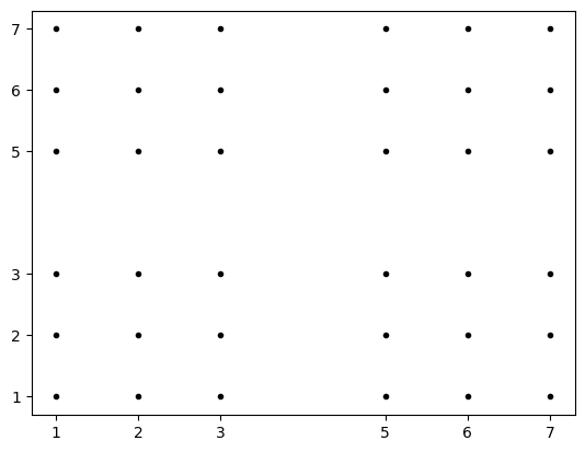

Remarks

1. Using meshgrid, we can create coordinate metrices x, y.
2. Meshgrid allows to make all possible combinations for given arrays elements.

Plotting two dimension functions

Sine function

def sin(x, y):
    return np.sin(x) + np.sin(y)

z = sin(x, y)
z

array([[ 0.79810661,  1.49845758,  1.56628403, -0.30193768,  0.3775711 ,
         1.3139732 ],
       [-0.13829549,  0.56205549,  0.62988193, -1.23833977, -0.558831  ,
         0.3775711 ],
       [-0.81780427, -0.11745329, -0.04962685, -1.91784855, -1.23833977,
        -0.30193768],
       [ 1.05041743,  1.75076841,  1.81859485, -0.04962685,  0.62988193,
         1.56628403],
       [ 0.98259099,  1.68294197,  1.75076841, -0.11745329,  0.56205549,
         1.49845758],
       [ 0.28224002,  0.98259099,  1.05041743, -0.81780427, -0.13829549,
         0.79810661]])

plt.figure(figsize=(8, 6))
plt.imshow(z, origin='lower')
plt.colorbar()
plt.locator_params(axis='y', nbins=4)
plt.locator_params(axis='x', nbins=4)
plt.show()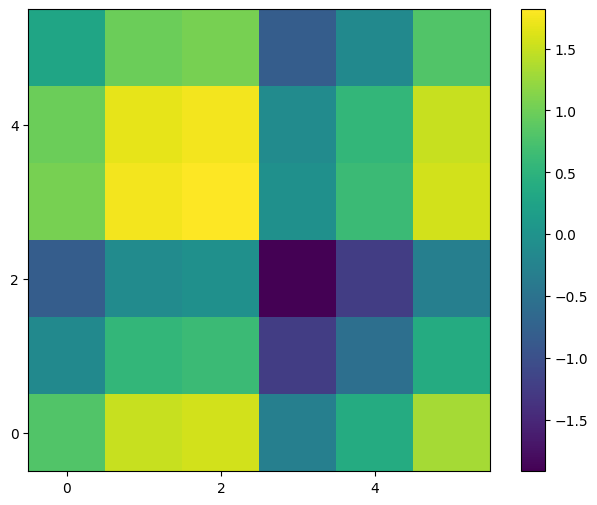

seq = np.linspace(-10, 10, 100)
x, y = np.meshgrid(seq, seq)

z = sin(x, y)

plt.figure(figsize=(8, 6))
plt.imshow(z)
plt.colorbar()
plt.locator_params(axis='x', nbins=4)
plt.locator_params(axis='y', nbins=4)
plt.show()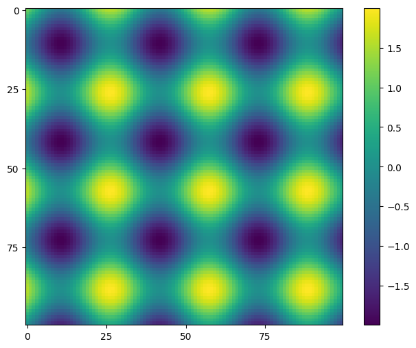

Another function

z = x ** 2 + (y - x) * 2

plt.imshow(z)
plt.colorbar()
plt.locator_params('x', nbins=4)
plt.locator_params('y', nbins=4)
plt.show()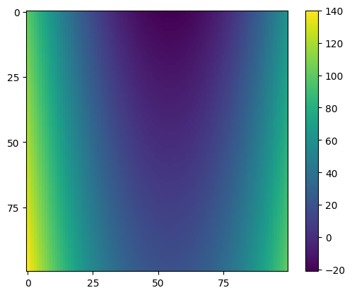

Plotting 3D functions

from mpl_toolkits.mplot3d import Axes3D

fig = plt.figure(figsize=(8, 4))
ax = fig.add_subplot(projection="3d")
 
ax.plot_surface(x, y, z)
plt.show()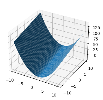

Approaching same problem without meshgrid

x2 = np.linspace(-10, 10, 100)[np.newaxis]
y2 = np.linspace(-10, 10, 100)[:, np.newaxis]

z2 = x ** 2 + (y - x) * 2
plt.imshow(z)
plt.colorbar()
plt.locator_params('x', nbins=4)
plt.locator_params('y', nbins=4)
plt.show()

Remarks

1. This approach is more memory efficient than using meshgrid because it has very less elements that meshgrid.

What about performance?

seq = np.linspace(-10, 10, 10000)
x, y = np.meshgrid(seq, seq)
 
%time x ** 2 + (y - x) * 2

CPU times: user 664 ms, sys: 421 ms, total: 1.09 s
Wall time: 1.09 s





array([[100.       ,  99.9559996,  99.9120072, ...,  59.9280088,
         59.9640004,  60.       ],
       [100.0040004,  99.96     ,  99.9160076, ...,  59.9320092,
         59.9680008,  60.0040004],
       [100.0080008,  99.9640004,  99.920008 , ...,  59.9360096,
         59.9720012,  60.0080008],
       ...,
       [139.9919992, 139.9479988, 139.9040064, ...,  99.920008 ,
         99.9559996,  99.9919992],
       [139.9959996, 139.9519992, 139.9080068, ...,  99.9240084,
         99.96     ,  99.9959996],
       [140.       , 139.9559996, 139.9120072, ...,  99.9280088,
         99.9640004, 100.       ]])

x2 = np.array([seq])
y2 = x2.T
 
%time x2 ** 2 + (y2 - x2) * 2

CPU times: user 442 ms, sys: 382 ms, total: 824 ms
Wall time: 847 ms





array([[100.       ,  99.9559996,  99.9120072, ...,  59.9280088,
         59.9640004,  60.       ],
       [100.0040004,  99.96     ,  99.9160076, ...,  59.9320092,
         59.9680008,  60.0040004],
       [100.0080008,  99.9640004,  99.920008 , ...,  59.9360096,
         59.9720012,  60.0080008],
       ...,
       [139.9919992, 139.9479988, 139.9040064, ...,  99.920008 ,
         99.9559996,  99.9919992],
       [139.9959996, 139.9519992, 139.9080068, ...,  99.9240084,
         99.96     ,  99.9959996],
       [140.       , 139.9559996, 139.9120072, ...,  99.9280088,
         99.9640004, 100.       ]])

Remarks

Performance is better than the meshgrid