spatial-frequency-notebook

import numpy as np
import matplotlib.pyplot as plt

def rgb_to_gray(rgb):
    r, g, b = rgb[:, :, 0], rgb[:, :, 1], rgb[:, :, 2]
    gray = 0.2989 * r + 0.5870 * g + 0.1140 * b
    return gray

Plotting grayscale image

todo;

choose the right two images to be used
plot two images sidewise
create amp and phase image for both images and plot them
create image by combining amp of first image and phase of second image and plot it

duck = "duck.jpg"
pattern = "pattern.jpg"

Images

duck_img = rgb_to_gray(plt.imread(duck))
pattern_img = rgb_to_gray(plt.imread(pattern))

plt.subplots(figsize=(16, 8))
plt.subplot(1, 2, 1)
img = plt.imshow(duck_img)
img.set_cmap('gray')
plt.subplot(1, 2, 2)
img = plt.imshow(pattern_img)
img.set_cmap('gray')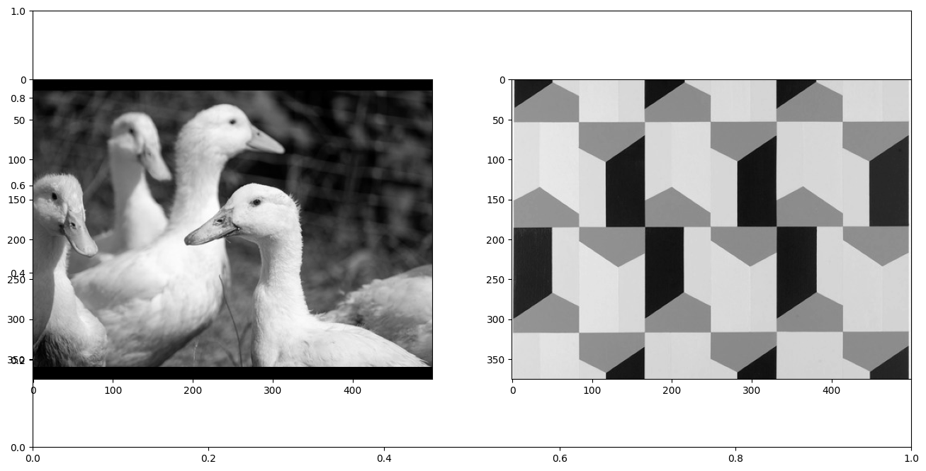

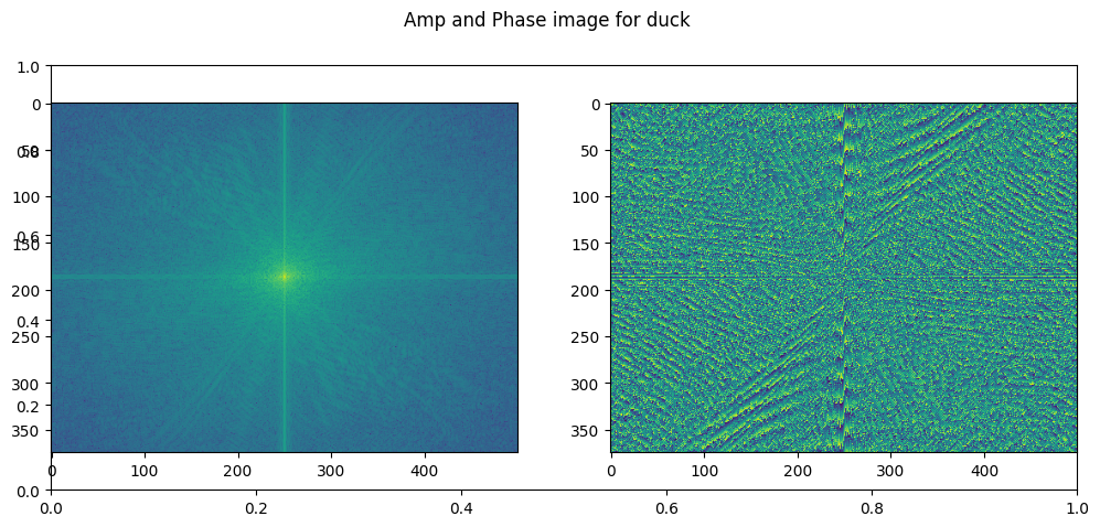
png

Apply fourier transformation on duck image

# duck_fft = np.fft.fft2(np.fft.fftshift(duck_img))
duck_fft = np.fft.fftshift(np.fft.fft2(duck_img))
plt.subplots(figsize=(12, 5))
plt.suptitle("Amp and Phase image for duck")
plt.subplot(1, 2, 1)
plt.imshow(10. * np.log10(np.abs(duck_fft)))
 
 
plt.subplot(1, 2, 2)
plt.imshow(np.angle(duck_fft))

<matplotlib.image.AxesImage at 0x7f2c2dda87c0>

png

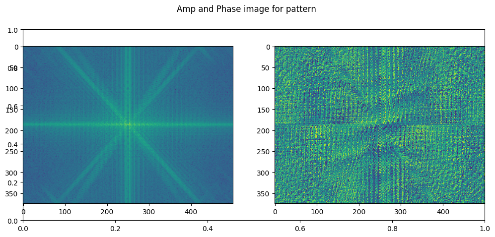
Apply fourier transformation on pattern image

pattern_fft = np.fft.fftshift(np.fft.fft2(pattern_img))
plt.subplots(figsize=(12, 5))
plt.suptitle("Amp and Phase image for pattern")
plt.subplot(1, 2, 1)
plt.imshow(10. * np.log10(np.abs(pattern_fft)))
 
plt.subplot(1, 2, 2)
plt.imshow(np.angle(pattern_fft))

<matplotlib.image.AxesImage at 0x7f2c300e8670>

png

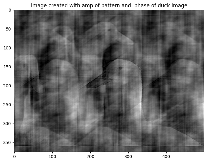
Create image using amp of pattern and phase of duck

amp = np.abs(pattern_fft)
phase = np.angle(duck_fft)
 
hybrid_ftt = amp * (np.cos(phase) + 1j * np.sin(phase))
 
# applying inverse fft
hybrid = np.abs(np.fft.ifft2(np.fft.fftshift(hybrid_ftt)))
 
 
plt.figure(figsize=(8, 8))
plt.title("Image created with amp of pattern and  phase of duck image")
img = plt.imshow(hybrid)
img.set_cmap('gray')

png

Create image using amp of duck and phase of pattern

amp = np.abs(duck_fft)
phase = np.angle(pattern_fft)
 
hybrid_fft = amp * (np.cos(phase) + 1j * np.sin(phase))
hybrid = np.abs(np.fft.ifft2(np.fft.fftshift(hybrid_fft)))
 
plt.figure(figsize=(8, 8))
plt.title("Image created with amp of duck and  phase of pattern")
img = plt.imshow(hybrid)
img.set_cmap("gray")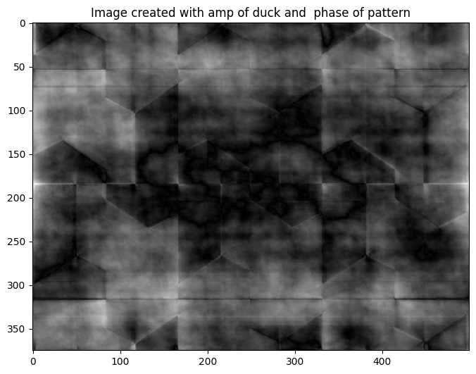

png

Remarks

Phase mostly defines the structures of the image. So, when phase of duck is used and amp of pattern, only the duck is visible.
When phase of pattern and amp of duck is used, we can only see the pattern.

Creating duck image using its phase and amp of all values 1.

phase = np.angle(duck_fft)
amp = np.ones_like(duck_fft)
 
phase_only_duck_fft = amp * (np.cos(phase) + 1j * np.sin(phase))
 
phase_only_duck = np.abs(np.fft.ifft2(np.fft.fftshift(phase_only_duck_fft)))
 
plt.figure(figsize=(8, 8))
plt.title("Duck phase only")
img = plt.imshow(phase_only_duck)
img.set_cmap("gray")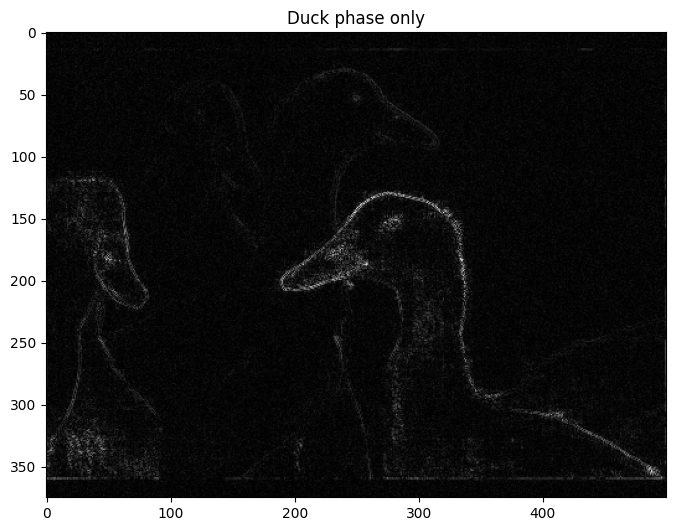

png

Creating duck image using amp only

amp = np.abs(duck_fft)
phase = np.angle(np.zeros_like(duck_fft))
 
amp_only_duck_fft = amp * (np.cos(phase) + 1j * np.sin(phase))
 
amp_only_duck = np.abs(np.fft.ifft2(np.fft.fftshift(amp_only_duck_fft)))
 
plt.subplots(figsize=(16, 8))
 
plt.suptitle("Duck image using amp only")
 
plt.subplot(1, 2, 1)
plt.title("Duck image")
img = plt.imshow(amp_only_duck)
img.set_cmap("gray")
 
# using decibles
 
amp = 10. * np.log10(np.abs(duck_fft))
amp_only_duck_fft = amp
plt.suptitle("Duck image using amp in dB")
plt.subplot(1, 2, 2)
img = plt.imshow(amp)
img.set_cmap("gray")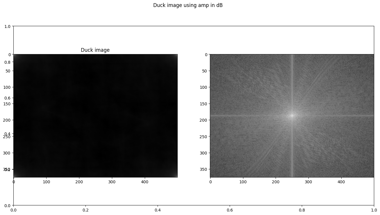

png

Creating duck images using real and imaginary components

duck_fft_real = duck_fft.real
duck_fft_imag = duck_fft.imag
duck_real = np.abs(np.fft.ifft2(duck_fft_real))
duck_imag = np.abs(np.fft.ifft2(duck_fft_imag))
 
 
plt.subplots(figsize=(12, 4.5))
plt.suptitle("Duck images using real and imaginary parts")
 
plt.axis("off")
plt.grid(False)
 
plt.subplot(1, 2, 1)
img = plt.imshow(duck_real)
img.set_cmap("gray")
 
plt.subplot(1, 2, 2)
img = plt.imshow(duck_imag)
img.set_cmap("gray")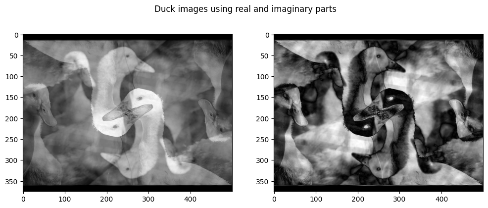

png

Plotting point source image

def point_source_fft(img_size, y_pos, x_pos, amp=1):
    point_img = np.zeros((img_size + 1, img_size + 1))
    
    point_img[y_pos, x_pos] = amp
    
    plt.subplots(figsize=(18, 8))
    plt.suptitle("Single point image")
    
    plt.grid(False)
    plt.axis(False)
    
    plt.subplot(1, 2, 1)
    plt.title("Single centered point image")
    plt.imshow(point_img, interpolation='nearest')
    plt.colorbar(shrink=0.8)
    plt.set_cmap("gray")
    
    ## not sure why fftshit is happening before fourier transformation here?? above images shows opposite of it.
    point_img_fft = np.fft.fft2(np.fft.fftshift(point_img))
    # point_img_fft = np.fft.fftshift(np.fft.fft2(point_img))
    
    phase = np.angle(point_img_fft)
    plt.subplot(1, 2, 2)
    plt.title("Phase")
    plt.imshow(phase)
    plt.colorbar(shrink=0.8)
    plt.set_cmap('hsv')

img_size = 128
x_pos = (img_size // 2) + 1
y_pos = (img_size // 2) + 1
 
point_source_fft(img_size, y_pos, x_pos)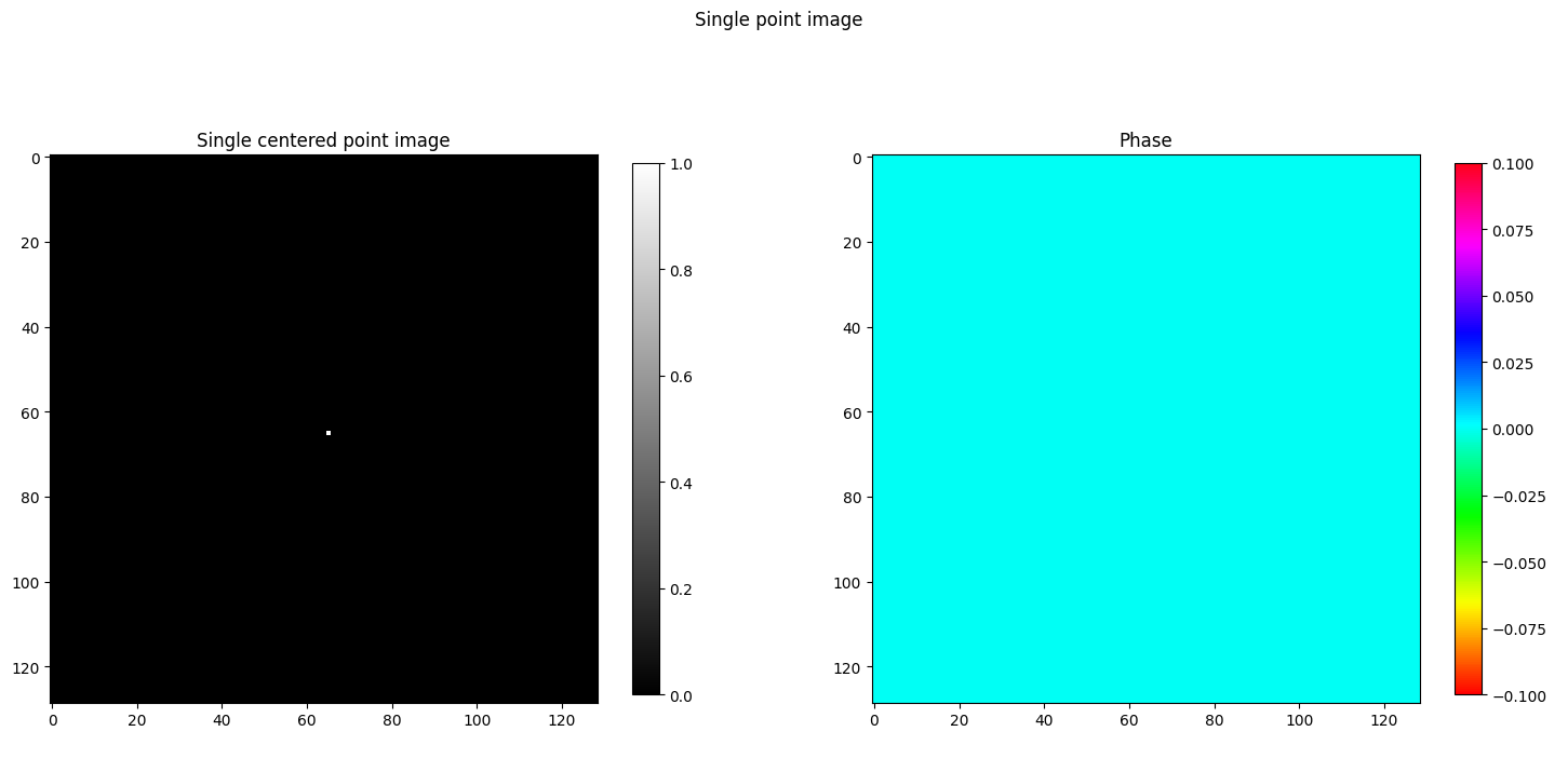

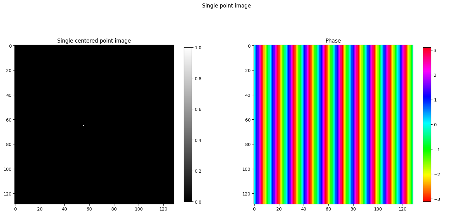
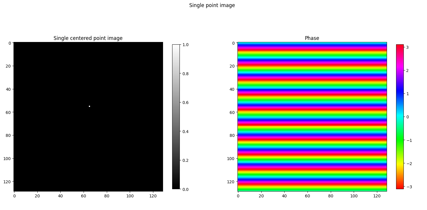
png

Phase fringe patterns on point location change from center

img_size = 128
point_source_fft(img_size, (img_size // 2) + 1, (img_size // 2))
 
point_source_fft(img_size, (img_size // 2) + 1, (img_size // 2) + 1 - 10)
 
point_source_fft(img_size, (img_size // 2) + 1 - 10, (img_size // 2) + 1)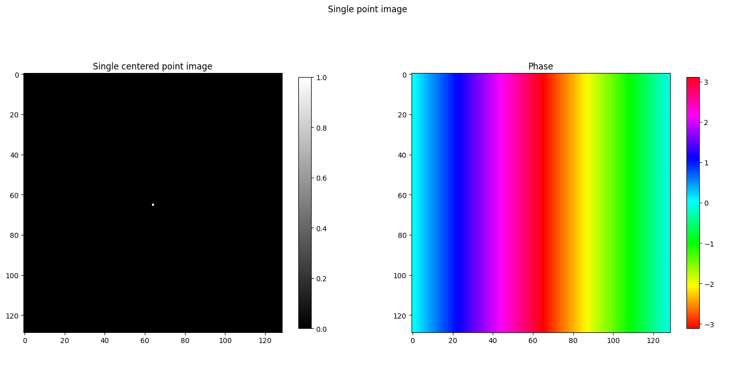

png

Remarks

So moving the point to left side, we get fringe color pattern for the phase.
Moving point vertically creates horizontal fringes.
Moving point horizontally creates vertical fringes.

Phase fringe pattern while rotating pixel around center

def point_source_fft_circle(img_size, y_pos, x_pos, amp=1., radius=10.):
    ## create image
    img = np.zeros((img_size + 1, img_size+2))
    img[y_pos, x_pos] = amp
    img_fft = np.fft.fft2(np.fft.fftshift(img))
 
    ## plot setup
    plt.subplots(figsize=(18, 8))
    plt.grid(False)
    plt.axis(False)
    
    ## image plot without fft
    ax = plt.subplot(1, 2, 1)
    plt.set_cmap("gray")
    plt.title("image without fft")
    plt.imshow(img, interpolation='nearest')
    plt.colorbar(shrink=0.8)
    circle = plt.Circle(((img_size/2)+1, (img_size/2)+1), radius, color='blue', linewidth=2, fill=False)
    ax.add_patch(circle)
 
    ## phase
    phase = np.angle(img_fft)
    plt.subplot(1, 2, 2)
    plt.title("image phase")
    plt.imshow(phase)
    plt.set_cmap("hsv")
    plt.colorbar(shrink=0.8)

img_size = 128
point_source_fft_circle(img_size, (img_size // 2) + 1 + 10, (img_size // 2) + 1)
point_source_fft_circle(img_size, (img_size // 2) + 1 + 10, (img_size // 2) + 1 + 10)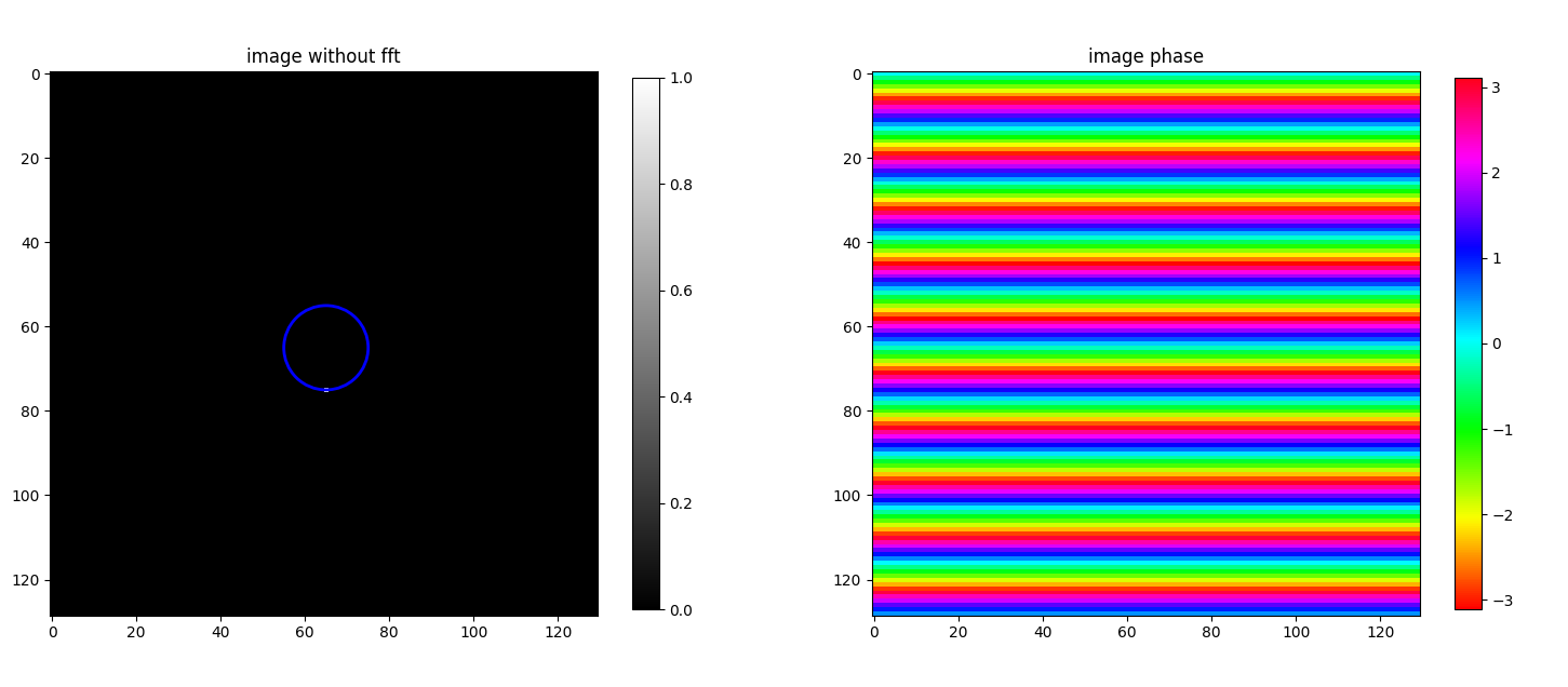

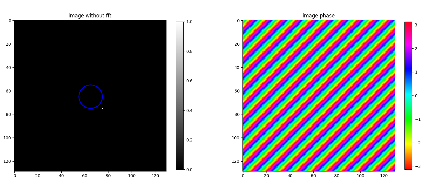
png

Remarks

When the pixel position rotates around the center without changing the distance, the phase frequency remains the same but the phase rotates.

FFT of multiple source points

def multiple_fft(img_size, pos, amps):
    img = np.zeros((img_size + 1, img_size + 1))
 
    ## fillup amps
    for p, a in zip(pos, amps):
        img[p[0], p[1]] = a
 
    img_fft_phase = np.angle(np.fft.fft2(np.fft.fftshift(img)))
    
    plt.subplots(figsize=(18, 8))
    plt.suptitle("multiple source points image")
    plt.grid(False)
    plt.axis(False)
 
    plt.subplot(1, 2, 1)
    plt.title("image")
    plt.imshow(img)
    plt.set_cmap('gray')
    plt.colorbar(shrink=0.8)
 
    plt.subplot(1, 2, 2)
    plt.title("phase")
    plt.imshow(img_fft_phase)
    plt.set_cmap("hsv")
    plt.colorbar(shrink=0.8)

imgSize = 128
 
multiple_fft(imgSize, [[64, 65], [90,80]], [1., 1])
multiple_fft(imgSize, [[64,65], [90,80], [40,10], [60,50], [20,80]], [.2, 0.3, 0.5, 0.1, 0.7])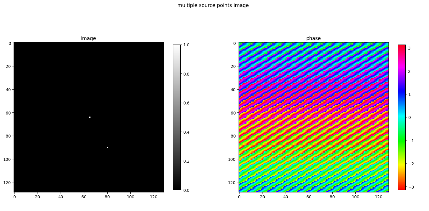

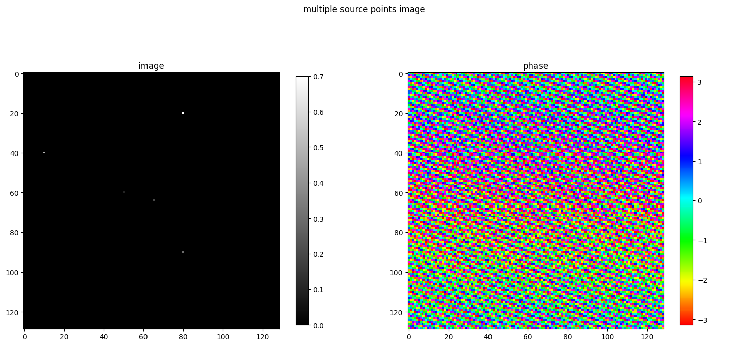
png

Remarks

Image with multiple sources has resulting phase an amplitude weighted average of phases of each point source.
It means that for the averaging of phases of each individual sources, their amplitudes are also taken into consideration.

Reconstructing duckk image

def reconstruct_image(vis, nsamples):
    new_vis = np.zeros_like(vis)
    y_pos = np.random.randint(0, high=vis.shape[0] - 1, size=int(nsamples))
    x_pos = np.random.randint(0, high=vis.shape[1] - 1, size=int(nsamples))
    
    new_vis[y_pos, x_pos] = vis[y_pos, x_pos] # substituting values
 
    img = np.fft.ifft2(np.fft.fftshift(new_vis))
    plt.subplots(figsize=(16, 6))
    plt.suptitle("Image reconstruction by taking samples")
    plt.grid(False)
    plt.axis(False)
 
    plt.subplot(1, 2, 1)
    plt.imshow(np.abs(new_vis).astype(bool), interpolation='nearest', cmap="gray")
    plt.title("sampled visibilities")
    
    plt.subplot(1, 2, 2)
    plt.imshow(np.abs(img), cmap="gray")
    plt.title("Reconstructed image")

reconstruct_image(duck_fft, 1e1)
reconstruct_image(duck_fft, 1e3)
reconstruct_image(duck_fft, 1e5)
reconstruct_image(duck_fft, 1e6)

png

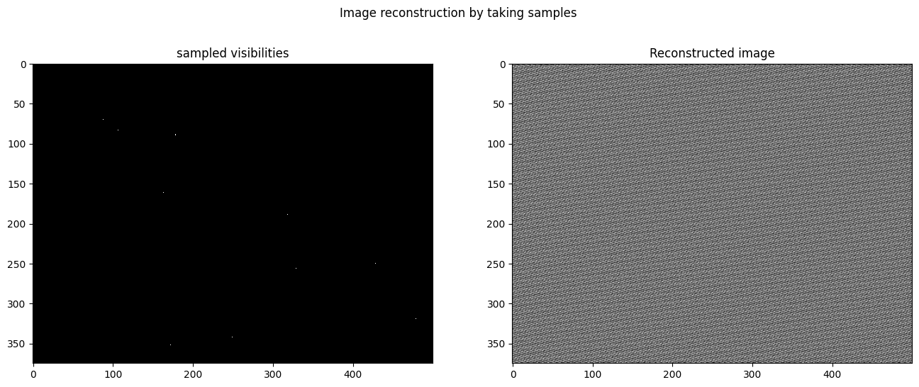
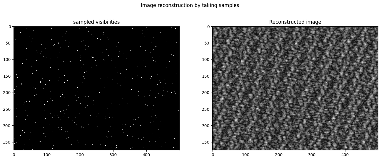
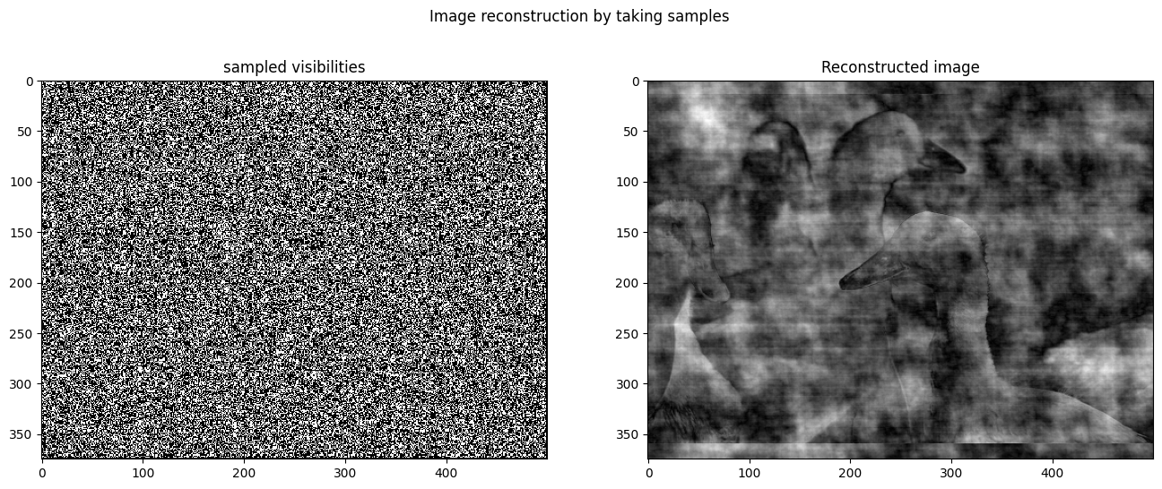
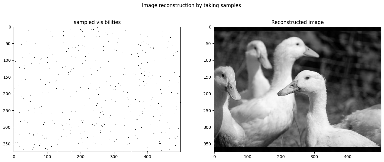
Remarks

We can recreate the image by selecting spatial frequencies with different amplitude and phases.
We don’t require to sample all the points to reconstruct the image.

bitPhile

Explorer

spatial-frequency-notebook

Plotting grayscale image

Images

Apply fourier transformation on duck image

Apply fourier transformation on pattern image

Create image using amp of pattern and phase of duck

Create image using amp of duck and phase of pattern

Remarks

Creating duck image using its phase and amp of all values 1.

Creating duck image using amp only

Creating duck images using real and imaginary components

Plotting point source image

Phase fringe patterns on point location change from center

Remarks

Phase fringe pattern while rotating pixel around center

Remarks

FFT of multiple source points

Remarks

Reconstructing duckk image

Remarks

Graph View

Table of Contents